

Summary of Key Points in This Article
- Article Difficulty: ★☆☆☆☆
- Tutorial on Running TQuant Lab in Google Colab
- Simple Test: Select the top five companies by revenue (from any industry) and backtest their returns
- Install fonts to ensure the Pyfolio package can plot graphs smoothly
Introduction
For students who want to use TQuant Lab, in addition to the original GitHub installation tutorial, we now offer a faster and simpler way to use it directly on Google Colab. The tutorial on running TQuant Lab in Google Colab eliminates the need to set up a virtual environment, significantly lowering the barrier to entry.
Running TQuant Lab in Google Colab and Installing some Commonly used Package
You only need one simple lines of code to complete the environment setup.
!pip install zipline-tejIf you encounter a pop-up window showing an error, simply click “Restart Runtime” to resolve it.
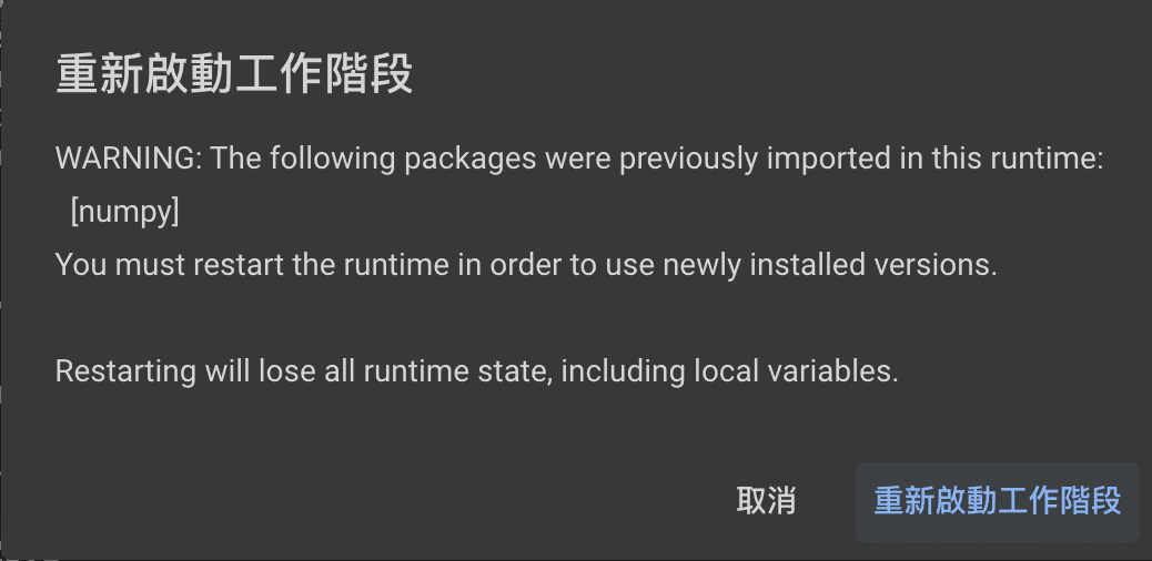
In the end, you may see the following error message, but you can ignore it. The system is actually ready for use.
ERROR: pip's dependency resolver does not currently take into account all the packages that are installed. This behaviour is the source of the following dependency conflicts.
cudf-cu12 24.4.1 requires pandas<2.2.2dev0,>=2.0, but you have pandas 1.5.3 which is incompatible.
google-colab 1.0.0 requires pandas==2.0.3, but you have pandas 1.5.3 which is incompatible.
TQuant Lab Tutorial: Selecting the Top Five Semiconductor Companies by Revenue for Backtesting
Load Commonly Used Packages
import os
os.environ['TEJAPI_BASE'] = 'https://api.tej.com.tw'
os.environ['TEJAPI_KEY'] = 'Your_Key'

import datetime

import tejapi
import pandas as pd
import numpy as np
First, identify all companies in the semiconductor
from zipline.sources.TEJ_Api_Data import get_universe

pool = get_universe(start = '2022-07-02',
                    end = '2023-07-02',
                    mkt_bd_e = 'TSE',
                    stktp_e = 'Common Stock',
                    sub_ind_e=['M2324 Semiconductor', 'M2325 Computer and Peripheral Equipment'])
Check their revenue and select the top five highest, then save their stock symbols.
import TejToolAPI

start_time = pd.Timestamp('2022-07-02')
end_time = pd.Timestamp('2023-07-02')

data = TejToolAPI.get_history_data(start = start_time,
                                   end = end_time,
                                   ticker = pool,
                                   fin_type = 'A',
                                   columns = ['營業總收入'],
                                   transfer_to_chinese = True)

data  = data.drop_duplicates(subset=['股票代碼'], keep='last').reset_index(drop=True)

data = data.nlargest(5, '營業總收入_A')    #select the top five highest

data| stock | date | Total_Operating_Income_A | |
|---|---|---|---|
| 6 | 2330 | 2023-06-30 | 508632973.0 |
| 90 | 4938 | 2023-06-30 | 318136546.0 |
| 27 | 2382 | 2023-06-30 | 266180950.0 |
| 67 | 3231 | 2023-06-30 | 212000207.0 |
| 4 | 2324 | 2023-06-30 | 209458784.0 |
tickers = data['股票代碼'].unique()Load the data onto your local computer.
start = '2023-07-03'
end = '2024-07-02'

os.environ['mdate'] = start + ' ' + end
os.environ['ticker'] = ' '.join(tickers) + ' ' + 'IR0001'

!zipline ingest -b tquant

from zipline.data import bundles
bundle_data = bundles.load('tquant')

from zipline.api import *
from zipline.finance import commission, slippage

def initialize(context):
    context.day = 0
    context.tickers = tickers
    set_slippage(slippage.VolumeShareSlippage(volume_limit = 0.025, price_impact = 0.1))
    set_commission(commission.Custom_TW_Commission(min_trade_cost = 20, discount = 1.0, tax = 0.003))
    set_benchmark(symbol('IR0001'))
    set_liquidity_risk_management_rule(['全額交割股票(Full-Cash Delivery Securities)', '漲停股票(Limit Up)', '跌停股票(Limit Down)', '開盤即鎖死(Limited Whole Day)'])

def handle_data(context, data):

    if context.day == 0:
        for ticker in context.tickers:
            order_percent(symbol(ticker), 1 / len(tickers))

    context.day += 1

import matplotlib.pyplot as plt

capital_base = 1e6

def analyze(context, results):

    fig = plt.figure()
    ax1 = fig.add_subplot(111)
    results['benchmark_cum'] = results.benchmark_return.add(1).cumprod() * capital_base
    results[['portfolio_value', 'benchmark_cum']].plot(ax = ax1, label = 'Portfolio Value($)')
    ax1.set_ylabel('Portfolio value (TWD)')

    plt.legend(loc = 'upper left')

    plt.gcf().set_size_inches(18, 8)
    plt.grid()
    plt.show()

from zipline import run_algorithm

start_date = pd.Timestamp('20230703', tz = 'utc')
end_date = pd.Timestamp('20240702', tz = 'utc')

results = run_algorithm(
    start = start_date,
    end = end_date,
    initialize = initialize,
    handle_data = handle_data,
    analyze = analyze,
    bundle = 'tquant',
    capital_base = capital_base,
)

results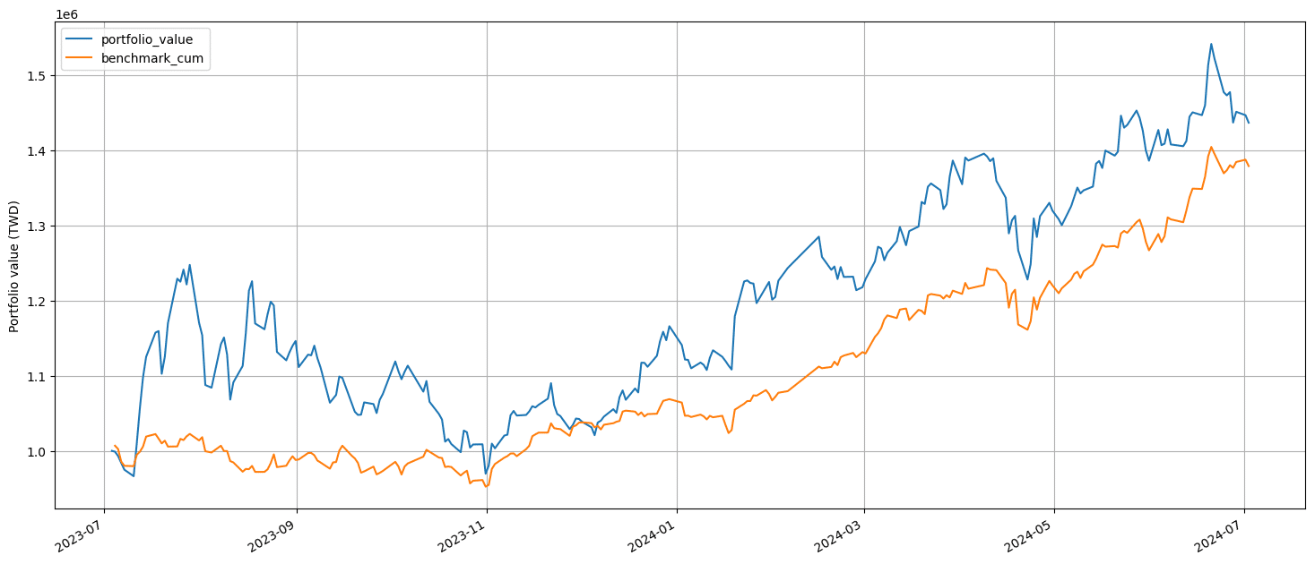
Font Issues Encountered with Pyfolio and How to Resolve Them
from pyfolio.utils import extract_rets_pos_txn_from_zipline
import pyfolio as pf

returns, positions, transactions = extract_rets_pos_txn_from_zipline(results)
benchmark_rets = results.benchmark_return

from pyfolio.plotting import plot_rolling_sharpe

plot_rolling_sharpe(returns, factor_returns=benchmark_rets)
WARNING:matplotlib.font_manager:findfont: Generic family 'sans-serif' not found because none of the following families were found: Microsoft JhengHei
WARNING:matplotlib.font_manager:findfont: Generic family 'sans-serif' not found because none of the following families were found: Microsoft JhengHei
WARNING:matplotlib.font_manager:findfont: Generic family 'sans-serif' not found because none of the following families were found: Microsoft JhengHei
WARNING:matplotlib.font_manager:findfont: Generic family 'sans-serif' not found because none of the following families were found: Microsoft JhengHei
WARNING:matplotlib.font_manager:findfont: Generic family 'sans-serif' not found because none of the following families were found: Microsoft JhengHei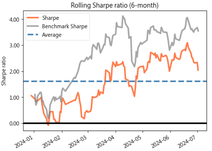
Even though the charts have been successfully plotted, you may still encounter warnings about missing fonts. To resolve this issue, you can manually load the fonts.
import matplotlib
import matplotlib.font_manager as fm
!wget -O MicrosoftJhengHei.ttf https://github.com/a7532ariel/ms-web/raw/master/Microsoft-JhengHei.ttf
!wget -O ArialUnicodeMS.ttf https://github.com/texttechnologylab/DHd2019BoA/raw/master/fonts/Arial%20Unicode%20MS.TTF

fm.fontManager.addfont('MicrosoftJhengHei.ttf')
matplotlib.rc('font', family='Microsoft Jheng Hei')

fm.fontManager.addfont('ArialUnicodeMS.ttf')
matplotlib.rc('font', family='Arial Unicode MS')
After trying again, the warning messages should no longer appear.
plot_rolling_sharpe(returns, factor_returns=benchmark_rets)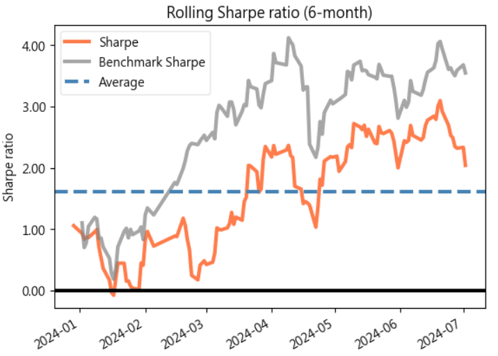
Conclusion
This introduction’s testing section mostly references the code from the article “TQuant Lab Warren E. Buffett’s Business Investment Rules.” You can refer to the original extended reading content if you have any questions.
Additionally, this introduction allows everyone to use TQuant without needing extra virtual environment installations and extensive settings. It’s much more convenient to get started right away and follow this recommended approach.
【TQuant Lab Backtesting System】Solving Your Quantitative Finance Challenges
Providing Comprehensive Tools for Trading Backtesting