
Use trial database to determine the weight of your portfolio.

Highlights
- Difficulty:★★★☆☆
- Calculate and visualize efficient frontier.
- Advise:This article will introduces the theory roughly. It will not be discussed in detail. Readers who are interested in theory can search for relevant literature. The mathematical calculations will be relatively complicated, using lot of functional programming to increase efficiency and reduce memory requirements. We use plotly module to visualize the result, and the interactive charts allow us to deeply understand the power of result.
Preface
Most people often have hard time to determine the weight of portfolio. However, Harry Markowitz, the Nobel Prize winner in economics, gives us a theory based on the volatility and correlation of stocks. Simulated by different weights on portfolio, we can put the restrictions like given the total risk is the same, to find the highest expected rate of return. In this way, we can choose the weight distribution of portfolio according to our own risk tolerance!
The Editing Environment and Modules Required
Mac OS and Jupyter Notebook
# basic
import numpy as np
import pandas as pd
# plot
import matplotlib.pyplot as plt
import matplotlib
import plotly.express as px
import plotly.graph_objects as go
# API
import tejapi
tejapi.ApiConfig.api_key = 'Your Key'
tejapi.ApiConfig.ignoretz = True
Database Used
- Trial Database : ‘ TRAIL/TAPRCD ’
Data Retrieval
Step 1. We use TSMC (2330), Evergreen (2603), and President Chain Store (2912) as examples of investment portfolios. The date is selected for 2020, and the option columns selected roi.
data = tejapi.get('TRAIL/TAPRCD',
                  coid=['2330', '2603', '2912'],
                  mdate={'gte': '2020-01-01', 'lte': '2020-12-
                          31'},
                  opts={"sort": "mdate.desc", 'columns': [
                        'coid', 'mdate', 'roi']},
                  paginate=True)
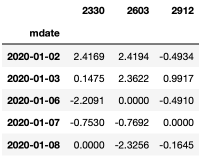
Step 2. Reset index value, data pivot, column name with stock code
data = data.set_index('mdate')
returns = data.pivot(columns='coid')
returns.columns = [columns[1] for columns in returns.columns]
Step 3. Calculate average return, covariance matrix
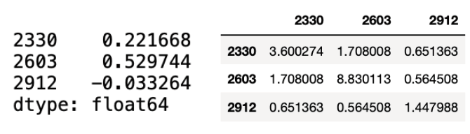
mean_returns = returns.mean()
cov_matrix = returns.cov()
Portfolio calculation
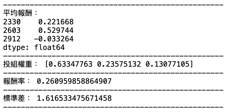
We need to randomly generate portfolio weights and use a large number of simulations to find the efficiency frontier. We need to record its return, standard deviation, and weight for each investment group.
def portfolio_performance(weights, mean_returns, cov_matrix):
    returns = np.sum(mean_returns*weights )
    std = np.sqrt(np.dot(weights.T, np.dot(cov_matrix, weights)))
    return std, returns
The number of portfolios we want to simulate.
num_portfolios = 5000
Put the function into the function which calculate random investment portfolio to get the results of each investment portfolio.
def random_portfolios(num_portfolios, mean_returns, cov_matrix):
    results = np.zeros((3,num_portfolios))
    weights_record = []
    for i in range(num_portfolios):
        weights = np.random.random(len(coid))
        weights /= np.sum(weights)
        weights_record.append(weights)
        portfolio_std_dev, portfolio_return =
        portfolio_performance(weights, mean_returns, cov_matrix)
        results[0,i] = portfolio_std_dev
        results[1,i] = portfolio_return
        results[2,i] = (portfolio_return) / portfolio_std_dev
    return results, weights_record
Start the simulation and save the results in results and weights_record
results = np.zeros((3,num_portfolios))
weights_record = []
for i in range(num_portfolios):
    weights = np.random.random(len(coid))
    weights /= np.sum(weights)
    weights_record.append(weights)
    portfolio_std_dev, portfolio_return =
    portfolio_performance(weights, mean_returns, cov_matrix)
    results[0,i] = portfolio_std_dev
    results[1,i] = portfolio_return
    results[2,i] = (portfolio_return) / portfolio_std_dev
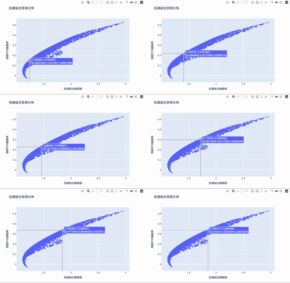
Visualization: The first number of the text box represents the risk, the second number represents the reward, and the second row of the array represents the weight of the investment.
def protfolios_allocation(mean_returns, cov_matrix,
                         num_portfolios):
    results, weights = random_portfolios(
        num_portfolios, mean_returns, cov_matrix)

    fig = go.Figure(data=go.Scatter(x=results[0, :],
                                    y=results[1, :],
                                    mode='markers',
                                    text = weights_record,
                                   ))

    fig.update_layout(title='投資組合表現分佈',
                      xaxis_title="投資組合總風險",
                      yaxis_title="預期平均報酬率",)fig.update_xaxes(showspikes=True,spikecolor="grey",
                     spikethickness=1, spikedash='solid')fig.update_yaxes(showspikes=True,spikecolor="grey",
                     spikethickness=1, spikedash='solid')fig.show()
Efficient Frontier
There are two conditions:
- The portfolio with the least risk among all portfolios
- Portfolio with minimal risk under the same rate of return
This type of condition is equivalent to finding the extreme value, we can use optimize under the scipy module to calculate the minimum value.
import scipy.optimize as sco
Here we define four calculation functions
Volatility
def portfolio_volatility(weights, mean_returns, cov_matrix):
 return portfolio_performance(weights,mean_returns, cov_matrix)[0]
Minimal Volatility Portfolio (MVP)
We use the optimize calculation under the scipy module to take the extreme value of the Volatility function under the weight limit of 0 to 1, and the algorithm selects SLSQP (Sequential Least Squares Programming) nonlinear programming
fun:objective function
args:parameters that can be set for the objective function
method:Optimal algorithm
bounds:Range of each x
constraints:the input is a tuple composed of a dictionary, the dictionary is mainly composed of’type’ and’fun’, type can be’eq’ and’ineq’, which are equality constraints and inequality constraints, respectively, fun is the corresponding constraint The condition can be a lambda function.
def min_variance(mean_returns, cov_matrix):
    num_assets = len(mean_returns)
    args = (mean_returns, cov_matrix)
    constraints = ({'type': 'eq', 'fun': lambda x: np.sum(x) - 1})
    bound = (0,1)
    bounds = tuple(bound for asset in range(num_assets))
    result = sco.minimize(portfolio_volatility, num_assets*
             [1/num_assets,], args=args,
             method='SLSQP', bounds=bounds,
             constraints=constraints)
    return result
MVP under the same rate of return
Mainly Due to the difference in constraint conditions, the returns should be fixed to a number, and find the minimum of risk.
def efficient_return(mean_returns, cov_matrix, target):
    num_assets = len(mean_returns)
    args = (mean_returns, cov_matrix)def portfolio_return(weights):
        return portfolio_performance(weights, mean_returns,
                                     cov_matrix)[1]constraints = ({'type': 'eq', 'fun': lambda x:
                     portfolio_return(x) - target},
                   {'type': 'eq', 'fun': lambda x: np.sum(x) - 1})bounds = tuple((0,1) for asset in range(num_assets))
    result = sco.minimize(portfolio_volatility, num_assets*
                          [1/num_assets,], args=args,
                          method='SLSQP', bounds=bounds,
                          constraints=constraints)
    return result
Sample after combined efficient frontier
def efficient_profolios(mean_returns, cov_matrix, returns_range):
    efficients = []
    for ret in returns_range:
        efficients.append(efficient_return(mean_returns,
                          cov_matrix, ret))
    return efficients
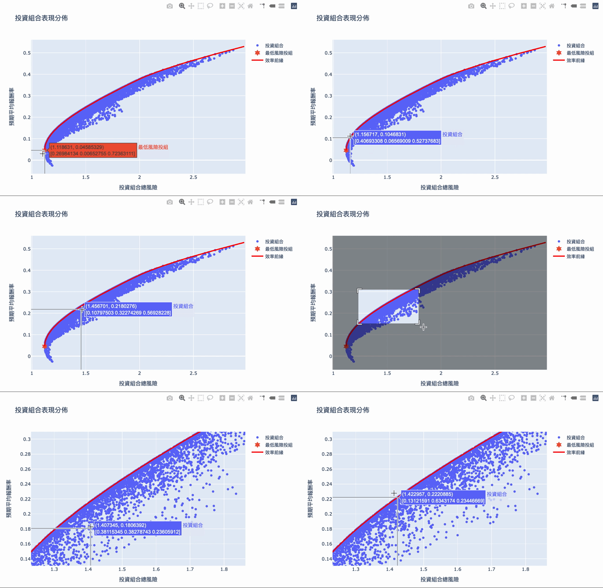
Conclusion
The overall structure of the efficient frontier is actually not difficult to understand. Using a large number of simulation calculations to obtain the weighted, you can set the expected return you want and choose the investment portfolio with the least risk. The Plotly interactive chart allows us to move the mouse on chart, it will show the weight distribution of the current investment portfolio. Of course, the truth remained unchanged is “High returns with high risks.” If you want a higher return on investment, you need to bear greater volatility. The result of these weights is based on the time of selecting the database, the volatility of the stock at that time, so the efficiency frontier obtained will continue to change over time, so the weight needs to be adjusted for a period of time.